What and how to measure - Static measurements

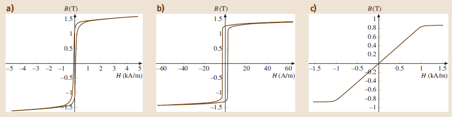
For quasistatic hysteresis measurements on soft magnetic materials, the DC hysteresisgraph or permeameter may be used.  Prior to the measurement the specimen is demagnetized. Often the measuring speed is controlled so that a constant rate of change of the flux density with time, dB/dt, is achieved. This allows the steep parts of the loop to be passed slowly to avoid errors due to eddy currents. The flat parts of the curves can be passed faster as eddy currents do not affect the magnetization.

Quasistatic measurement allows one to obtain magnetic material properties independently of the influence of eddy currents. In this way the hysteresis loss can be obtained directly by integrating the area of the hysteresis loop.

Coercivities of soft magnetic ring specimens range from less than 0.1A/m for ring cores made of wound ribbons of amorphous alloys up to several 100A/m for rings made of solid steel or sintered material. Depending on the ring dimensions, current and number of primary turns, typically maximum field strengths up to  approximately 10 kA/m can be achieved.

The permeability curve μ_r(H) can be created by dividing the corresponding values of B and μ₀H, which are usually taken from the initial magnetization curve. The highest point of the μ_r(H) curve, the maximum permeability μ_max, is typically stated in measurement reports.

Figure shows some sample measurements on different materials. The field strength excitation is 5kA/m for the Fe–Si and 60A/m for the Fe–Ni specimen.

Article src: Handbook of Materials Measurement Methods, Horst Czichos, Tetsuya Saito, Leslie Smith, Springer Science+Business Media, 2006.

The VSM allows relatively fast measurements (1–10min for a complete M(H) loop, depending on the type of magnet and the required sensitivity), is flexible and easy to use. In particular, measurements at various angles can be made with the great precision required for the determination of magnetic anisotropies. The sensitivity attainable depends largely on the geometry and position of the pick-up coils. Standard versions are useful for magnetic moments corresponding to Fe or NiFe films more than 5 nm thick (assuming a lateral size of 1–2 cm). Thinner films down to 1 nm can be measured with an optimized VSM. The sensitivity is generally reduced for variable-temperature measurements when a cryostat or oven must be mounted.

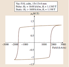
Room-temperature hysteresis loop as obtained on a cube of Vacodym 510 (an Nd–Fe–B magnet).

Pulsed Field Magnetometer (PFM) is a instrument that is well suited for fast and reliable measurement of the hysteresis loops of hard magnetic materials. The pulse magnet has to be optimized with respect to the available power, the heating of the magnet and the stresses. The field homogeneity over the desired length of the experiment should be better than 1%.

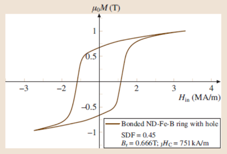
Hysteresis loop of a cylindrical sample with a hole of plastic-bonded Nd–Fe–B-type material.

For an industrial system a reasonable sample size is important; typical values are samples up to 30mm in diameter and 10mm in length within a ±1% pick-up homogeneity range. For magnetic measurements exact positioning (reproducibility better than 0.1mm) in the PFM is necessary

Article src: Handbook of Materials Measurement Methods, Horst Czichos, Tetsuya Saito, Leslie Smith, Springer Science+Business Media, 2006.

Generally the magnetocrystalline anisotropy constants are determined from measurements on a single crystal in a torque magnetometer or similar device. Unfortunately single crystals are not available from many materials.

In this case, polycrystalline material can sometimes be aligned in an external field and then the magnetization M(H) is measured parallel and perpendicular to the external field. Curves determined in this way can be fitted, which also allows an estimate of the magnetocrystalline anisotropy to be made.

If the magnetization energy of a freely rotating specimen depends on direction, the specimen aligns with its axis of easy magnetization parallel to a magnetic field. The axis of easy magnetization is determined by the magnetocrystalline anisotropy energy Eα if the specimen has rotational symmetry.

If the magnetic field is rotated out of the preferred direction by an angle α, the vector of polarization Js will point in the direction of H, if the field strength is sufficiently large to saturate the specimen. If H is smaller, the direction of Js is rotated only by an angle ϕ <α.

The specimen is attached to a rod that is suspended between torsion wires,  and is located between the poles of an electromagnet. The electromagnet is mounted to a base plate that can be rotated by 360◦. The rotation angle can be measured and recorded. The excitation of the specimen is measured by the deflection of a light beam from a mirror that is attached to the specimen rod.

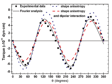
Magnetic torque measurements shown in Figure were performed by varying the angle θ between the applied magnetic field (9 kOe in amplitude) and the longitudinal axis of Ni nanowires array. Experimental data were well fitted by a Fourier series. As observed, the Fourier line fit displays a twofold symmetry that denotes the uniaxial character of the magnetic anisotropy. The fitted anisotropy constant gives a value of 5.7×10⁵ erg/cm³, indicating also that the magnetization easy axis lies parallel to the nanowires axis. Meanwhile, the plane of the sample substrate remains as a hard axis plane.

Article src: Handbook of Materials Measurement Methods, Horst Czichos, Tetsuya Saito, Leslie Smith, Springer Science+Business Media, 2006.

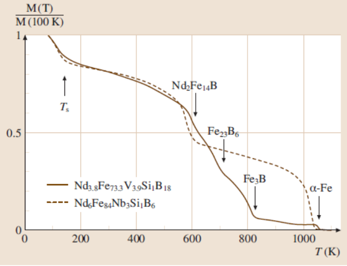
Curie temperature (T_C), or Curie point, is the temperature above which certain materials lose their permanent magnetic properties. The Curie temperature is usually obtained by differentiating of the temperature magnetization curves or by analyzing the critical behavior of magnetization at temperature, close to but lower than the Curie point.

Knowledge of the temperature dependence of the magnetic moments and the anisotropy energies is necessary for a correct interpretation of the measurements. Temperature dependencies are usually derived from bulk magnetic properties. The magnetic properties of small particles, however, are strongly influenced by surface effects related to low-temperature oxidation, reduced coordination of surface spins and interactions with surrounding molecules.

Figure shows measurements VSM on nanocrystalline specimens. Measurement below room temperature was carried out using an LN₂ cryostat. Above room temperature a tubular oven was used; it had a water-cooled outer wall to avoid heating of the pick-up coils and electromagnet poles. The oven can be evacuated or filled by an inert gas to avoid specimen oxidation.

Article src: Handbook of Materials Measurement Methods, Horst Czichos, Tetsuya Saito, Leslie Smith, Springer Science+Business Media, 2006.

In order to calculate the temperature dependence of the magnetic response for magnetic nanoparticles  systems (MNPs), it is necessary to consider the effect of thermal fluctuations that allow transitions between stable configurations. Doing so, it is possible to simulate M vs. T experiments as the extensively performed Zero Field Cooling-Field Cooling (ZFC-FC) routine. In this kind of experiment, a sample is cooled from a temperature where all particles show superparamagnetic behaviour to the lowest reachable temperature (typically ≤ 10 K), then, a small constant field usually lower than 8 kA/m is applied, and the sample is heated to a temperature high enough to observe an initial growth and subsequent decrease of its magnetization, i.e., up to the temperature range where the sample shows again superparamagnetic behaviour. The sample is then cooled again to the lowest temperature with the constant field still applied.

In the ideal case of a monosized non interacting MNPs sample, a narrow temperature region should exist in which the system performs a transition between irreversible and reversible regimes. When heating under an applied field, the thermal energy kT is initially much smaller than the anisotropy barrier KV so the magnetization remains null. Due to the exponential dependence of the Néel relaxation time with temperature (τ_~ e^kV/kBT), when kT ∼ KV, the magnetization grows rapidly up to its thermodynamic equilibrium value. Blocking Temperature T_B can be considered as the inflection point (IP) of this growing, or even a well defined maximum in ZFC branch (left figure) and its experimental determination is an important goal of the MNPs characterization.

Real samples always present a size dispersion, usually reasonably well described by a log-normal distribution. Different particle size implies a different anisotropy barrier KV and therefore a different T_B for each size fraction, so in real ZFC-FC experiments, the blocking region is wide and a representative T_B value of the ensemble is not well defined. An alternative approach is depicted in right figure where the T_B distribution is obtained from the T derivative of the difference between FC and ZFC curves.

Eventually, the blocking temperature  may also be approximated by    where  is the Boltzmann constant,   is the magnetic anisotropy energy, assuming an average volume value.

Article src: Bruvera et al. [J. Appl. Phys. 118, 184304 (2015)].