It all started like this - Everyday Applications

It is generally admitted that the magnetic fields of the Earth and other heavenly bodies are produced by motion of a conducting fluid core, although the details are mired in controversy. In the Earth’s case, the liquid core has inner and outer radii of 1220 and 3485 km, respectively, and is made of molten iron with minor amounts of nickel and other elements which have no strong affinity for oxygen. Less electronegative elements form oxides, which end up in the mantle.

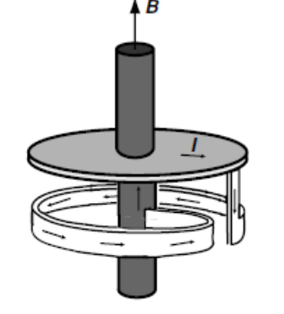
An important step towards understanding the origin of the Earth’s magnetic field was the concept of a self-sustaining fluid dynamo suggested by Joseph Larmor in 1919. A mechanical model of a self-exciting dynamo is a spinning conducting disc connected to a single-turn coil. If there is some small field to begin with, an emf is generated between the axle and the rim of the spinning disc, which drives current around the circuit, thereby building up the field. The basic idea is that the fluid motion somehow stretches and twists the flux lines, thereby intensifying the magnetic field. Just how this applies to the Earth is a matter for debate, but some constraints have been established.

One is that the dynamo cannot be axially symmetric. Another is that the field in the core is quite different from the poloidal, dipolar field observed at the surface. It is thought to have a pronounced azimuthal character, generated by differential rotation between the liquid core and the mantle. The azimuthal field is generated by poloidal currents in the liquid core. In one model of the geodynamo, turbulence leads to small-scale reorganization of the azimuthal field which creates the dipolar field.

Article src: Magnetism and Magnetic Materials, J. M. D   Coey,  Cambridge University Press, 2010.

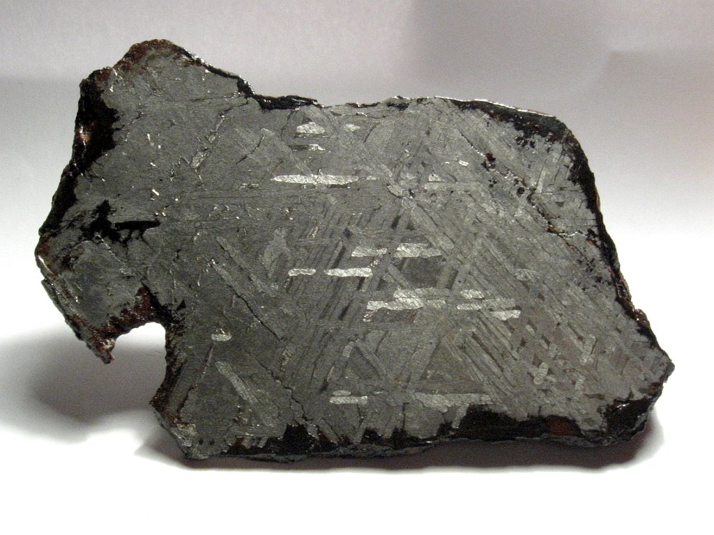
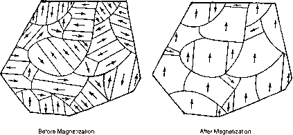
Iron meteorite may not be a material of choice for magnetic device applications, nevertheless it has its place in the study of the solar system. As such, planetary scientists may have an interest in the Widmanstatten structure that was formed by the long range diffusion of Fe and Ni in an asteroid’s core over a period of 4.6 billion years. This remarkable formation process has resulted in unusual magnetic properties not observable in synthetic Fe–Ni alloys. It should be noted that the Widmanstatten structure is regarded as Fe–Ni alloy segregated ˛ α (bcc Fe– Ni) and γ (fcc Fe–Ni) lamellae on a micrometer scale where the Ni concentration

In the γ lamellae increases rapidly toward the interface. The Widmanstatten structure is assumed to be responsible for the large magnetic anisotropy and strong coercivity displayed in iron meteorites which are a special type of Fe–Ni alloy. In this unique alloy, a tetrataenite phase is formed, described as a chemically ordered Fe–Ni alloy with L1₀-type superstructure. This phase was found to have an unbelievably large coercive force, and also a magnetic anisotropy energy that is one order of magnitude larger than that of Fe, permalloy, or pure Ni. As such, iron metoerite is a hard ferromagnet with a strong anisotropy, in spite of the fact that common Fe–Ni alloys are soft ferromagnetic materials. A transversal striped domain structure was observed in the α lamellae of the iron meteorite material, in contrast to the wide rectangular domain structure with a sharp domain wall, normally displayed by bcc-Fe.

Article src: Magnetism: Basics and Applications, Stefanita, Carmen-Gabriela, Springer Heidelberg Dordrecht London New York, 2012.

For centuries there had been dreams of magnetic levitation, i.e., the stable suspension in the air of a body made of iron or other magnetic material, without physical contact, by an artful arrangement of magnets exerting the proper attraction and repulsion. But such hopes were dashed in 1839 when S. Earnshaw proved that it could not be done. His theorem relates to both electrostatic and magnetostatic forces, or to any system of particles which exert forces on one another varying inversely as the square of the distance. For magnetic systems, Earnshaw’s theorem may be stated as follows: Stable levitation of one body by one or more other bodies is impossible, if all bodies in the system have a permeability greater than 1.

Stable levitation can be achieved for a positive permeability material if a position detector and feedback system are employed so that the force acting on the floating object is continuously adjusted, usually by varying the current through an electromagnet. This is the basis for various floating novelty items as well as for nearly zero-friction suspensions for various kinds of rotating instruments and machines.

If diamagnetic materials are included in the system, stable levitation becomes possible without power input. Levitation of this kind is easiest with a perfect diamagnet, namely, a superconductor. Figure shows a bar magnet floating over the slightly concave surface of superconducting lead at 4K. The magnet is in effect supported by its own field, which cannot penetrate into the lead.

The permeability of a superconductor is zero, and there are many diamagnetic materials with permeabilities slightly less than unity. But there are no diamagnetic materials with intermediate values of m, like 20.5. This means that only very light bodies, a few grams in weight, can be stably levitated at room temperature with the help of ordinary diamagnetic materials, like graphite or bismuth, because their flux-repelling powers are so feeble.

Quite large weights can be supported by the repulsion between permanent magnets, the lower one fixed to a base and the upper one to the underside of the load. Some lateral constraint is needed to make the load stable, but it need not be strong. The magnets must have high coercivity. Barium ferrite and rare-earth magnets are well suited to this application since they can be made in flat pieces of fairly large area, magnetized in the thickness direction.

Article src: Magnetism and Magnetic Materials, J. M. D   Coey,  Cambridge University Press, 2010.

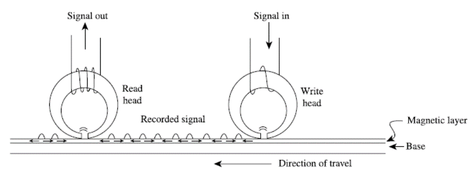
The basic arrangement for analog magnetic recording on tape, as well as for digital magnetic recording on tape and on disk, is shown in figure. A flexible or rigid substrate coated with a magnetic layer is moved past a write head, which is effectively a miniature electromagnet. A current in the winding of the write head magnetizes the head material, which creates a magnetic field in the head gap. The fringing field from the gap magnetizes the tape material in a pattern that reproduces the information to be recorded. The information is recorded in a stripe, called a track, running parallel to the length of the tape or in a circular path on a disk.

To read back the recorded information, the recorded track passes under a read head, which is similar to the write head. In low-cost audio recorders, the same head may be used for both reading and writing. The fringing magnetic field from the recorded tape magnetizes the read head as it passes by the head gap, and the changing magnetization in the head generates a signal voltage in the head winding. This voltage contains the recorded information, and can be amplified to recreate the recorded sound or video. Note that since the read head coil voltage is proportional to the time derivative of the flux change in the head, the amplification must include an integration step.

Article src: Introduction to Magnetic Materials (2nd Edition),  B. D. Cullity, C. D. Graham, Wiley-IEEE Press, 2008.

Claims of beneficial effects of static or low-frequency magnetic fields in pain relief and treatment of inflammation are controversial. It is thought that broken bones may set more quickly if they are exposed to a magnetic field. Unfortunately, no plausible explanation of such effects has yet been advanced.

Pulsed magnetic fields can be used to induce electric fields and drive currents in conducting tissue. The effects of transcranial magnetic stimulation of the brain using trains of pulses with dB/dt ≈ 10³−10⁶ T s⁻¹ are under investigation, and there is evidence that it may be beneficial in the treatment of neurological and psychiatric conditions such as Parkinson’s disease and depression. The pulses can induce weak emfs (nV–μV) at a cellular level, but the effects on the scale of an organ are more significant, because the induced electric fields increase in proportion to the dimensions.

Life on Earth has evolved in the presence of a weak magnetic field of 10– 100Am⁻¹. Inevitably, some creatures besides ourselves have learned to take advantage of this field. The clearest examples are magnetotactic bacteria, unicellular organisms which manufacture particles of ferromagnetic iron oxides (magnetite or maghemitite) or sulphides (greigite). The particles grow in chains in the microbe’s body. Each one is of a size which would make it superparamagnetic if it stood alone, but the anisotropic dipole–dipole interaction in a chain of particles stabilizes the magnetization direction along the chain. Thus, every bacterium has a built-in compass needle, which is handed on to the next generation with the polarization direction intact, by cellular division. New particles added to the ends of the half-chain grow in the stray field there, and become magnetized parallel to their neighbours.

Epidemiologic studies of human exposure to low-frequency fields from power lines or domestic wiring have proved inconclusive. Large static magnetic fields seem to be innocuous, with exposure provoking little response at the level of the organism. Studies of the influence of high-frequency fields from mobile phones have provided no clear evidence of harm.

Article src: Magnetism and Magnetic Materials, J. M. D   Coey,  Cambridge University Press, 2010.

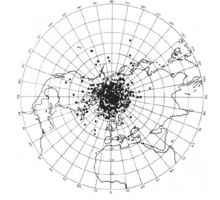
The ancient record of the Earth’s field has been inferred from the natural remanence of dated basalts. A first observation is that the direction of magnetization of young rocks indicates a magnetic pole direction that scatters randomly around the geographic axis. ‘Young’ for rocks is a few million years. The secular variation of the Earth’s field has been measured in Paris since 1600, but the record can be extended back to Roman times by measuring the thermoremanence of baked clay in the hearths of pottery kilns, which retain a record of the field direction on the last day they were used – a nice example of archaeometry, the use of quantitative physical methods in archaeology. Radiocarbon dating is used for these comparatively recent events. The secular variation seems to be a random wander around the Earth’s axis of rotation.

The most remarkable fact is that the polarity of the Earth’s field has flipped randomly over geological time. Half the points in figure are normal (present-day) polarity and half are reversed. The last reversal took place 700 000 years ago, and the polarity of the Earth’s field is subject to more-or-less random changes on timescales of 10⁵−10⁶ years. A sequence of lavas shows a characteristic pattern of normal and reversed polarity, providing the record of recent reversals. Altogether some 400 reversals have been recorded in the rock records. The dipole field at a reversal changes sign over a period of a few thousand years, during which time the nondipole, higher-order harmonics are thought to be dominant. We are unable to predict these reversals. As with stock markets, past record is no guide to future performance.

Article src: Magnetism and Magnetic Materials, J. M. D   Coey,  Cambridge University Press, 2010.

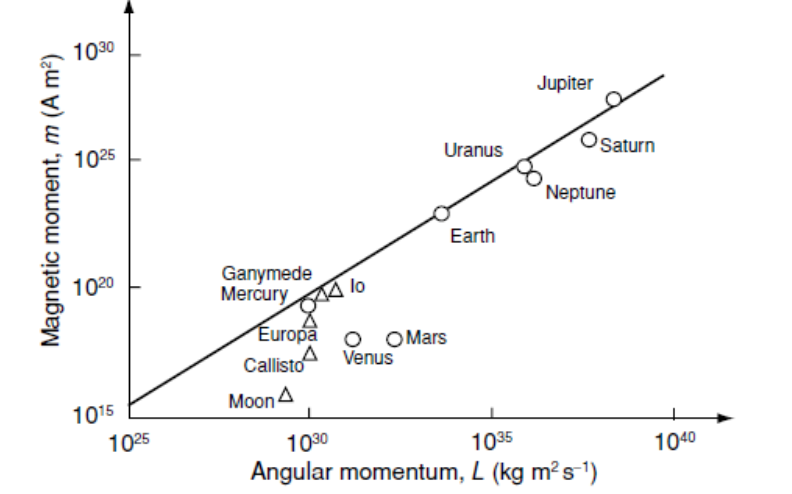
The planets and moons of our solar system have been investigated with the help of magnetometers on board spacecraft. Measurements show that their magnetic moments are mostly proportional to their angular momenta, a relation known as Busse’s law. The moments are almost always directed along the axis of rotation which suggests a dynamo effect in a conducting core. The core in the gas giants is likely to be a high-pressure metallic form of hydrogen rather than molten Fe–Ni, as in Earth. The magnetic field at the surface of Jupiter is ten times as strong as that at the surface of Earth, and its magnetic moment is roughly 20 000 times as large. The weak fields of the Moon and Mars are probably related to the absence of any liquid core.

Article src: Magnetism and Magnetic Materials, J. M. D   Coey,  Cambridge University Press, 2010.

Iron represents about 5% of the mass of the continental crust, and it is present in most rocks. Other magnetic elements are far scarcer.

Taking account of the fact that the atomic weight of iron is 2.2 times the crustal average we have the 40:40 rule: iron represents about 1/40 th of the atoms of the crust, and it is 40 times as abundant as all the other magnetic atoms together. Rocks are normally diamagnetic when they contain less than about 0.2 wt% iron, and paramagnetic otherwise, due to the presence of Fe²⁺ and Fe³⁺ ions in the crystal lattices of the mineral phases at concentrations well below the percolation threshold.

Applications of rock magnetism are based on measurements of the natural remanence, which can be acquired in several ways. Most important is the thermoremanent magnetization, acquired when igneous or metamorphic rocks cool through the superparamagnetic blocking temperature of the titanomagnetite grains. Rocks often have complex thermal and geological histories, and components of the remanence with differing stability can be acquired at different times in their past. Natural remanent magnetization can range from 10⁻⁵  to 10² Am⁻¹. Weaker remanence is acquired when grains sediment in the Earth’s field, or when they grow to exceed the critical blocking size as a result of some low-temperature chemical process.

Article src: Magnetism and Magnetic Materials, J. M. D   Coey,  Cambridge University Press, 2010.

The high-frequency applications of soft ferrites are mainly as cores for special transformers or inductors. Certain communication equipment requires broadband transformers; as the name implies, they must have cores that show the same behavior over a broad range of frequencies. Another application is in pulse transformers. Because the Fourier components of a square pulse extend over a wide range of frequencies; excessive distortion of the pulse shape occurs if the permeability of the core varies with frequency. Built-in ferrite antennas are much used in modern radio receivers. Such an antenna is merely a ferrite rod wound with a coil. It responds to the magnetic component of the incident electromagnetic wave, and the alternating flux in the ferrite induces an emf in the coil; the ferrite core in effect multiplies the area enclosed by the coil by a factor equal to the permeability. Finally, there are important microwave applications of ferrites, both in communications and in radar circuits. These involve frequencies of some 10¹⁰ Hz.

Article src: Introduction to Magnetic Materials (2nd Edition),  B. D. Cullity, C. D. Graham, Wiley-IEEE Press, 2008.

Although soft iron can be purified and made into an attractive material with high permeability and low coercive force, the cost of processing would be so high that it is only used in certain special applications. One area in which soft iron with moderate amount of impurities is sometimes applied is in electromagnets. The ultra high purity is not necessary in this and other applications. Areas where lower purity soft iron may be used include DC relays, plungers, pole pieces, solenoids and brakes for intermittent use where the magnetic requirements are low and the cost must be low.

In most cases, the iron is used in the bulk form (sintered or wrought) since Eddy currents are not operative at DC Soft pure iron is not really appropriate for AC applications because of its low resistivity.  As substitutes for soft iron, the next materials with improved properties at low frequencies are the low carbon steels.

In most applications ultra-high-purity iron is unnecessary. A typical commercial soft iron for electromagnet applications will therefore contain about 0.02% C, 0.035% Mn, 0.025% S, 0.015% P and 0.002% Si in the form of impurities. The magnetization curves of high-purity iron and a commercial soft iron after annealing in hydrogen to remove impurities are shown in figure.

For electromagnets the principle question that arises is what field is necessary to produce an induction of 1.0 Tor 1.5 T. For the commercial soft iron given above the values are typically 200 A/m and 700 A/m, respectively. Any form of mechanical deformation will result in a deterioration of the magnetic properties of soft iron for electromagnet applications. The internal stresses produced by such cold working can be removed by annealing at temperature between 725°C and 900°C providing the material does not suffer oxidation during the anneal which would also result in impaired magnetic properties. The usual procedure now is to anneal in a hydrogen atmosphere which has the additional advantage of removing some of the impurities

Article src: Handbook of modern ferromagnetic materials, A. Goldman, B.S., Springer Science+Business Media New York, Ferrite Technology Worldwide, (1st edition), 1999.

Article src: Introduction to Magnetism and Magnetic Materials (1nd edition), David Jiles, Chapman & Hall/CRC, 1991.

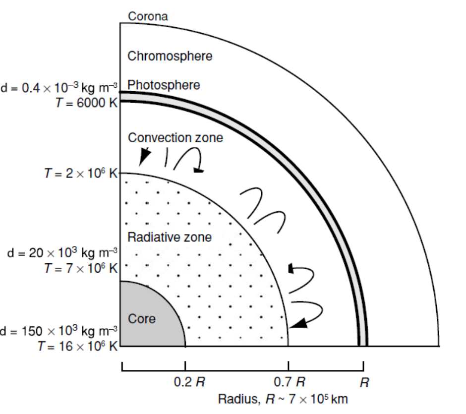
The ambient magnetic field in interplanetary space is 1–10 nT, whereas in interstellar space it is estimated to be 0.1 nT. The average field at the surface of the Sun is 100 μT, comparable to that at the surface of the Earth, but it can rise to over 100 mT in sunspots.

The surface of the Sun, is less dense than air on Earth but it is seething with activity. It has a granular appearance, due to a network of convection cells, each about 10³ km in diameter. The cells are bright at the centre, where hot plasma rises to the surface, and dark at the edges, where cooler plasma descends. The average surface temperature is 5800 K. Solar flares are spectacular displays leaping 10⁵ km out from the surface. They are accompanied by ejection of bursts of energetic particles, boosting the solar wind which streams outwards from the Sun, taking about two days to reach Earth.

Particle fluxes here are 10¹²–10¹³ m⁻² s⁻¹. Thankfully, these energetic charged particles are deflected by the Earth’s magnetic field high above the surface, but some find their way towards the Earth at high latitudes where they dissipate their energy in collisions in the ionized upper atmosphere. The green glow of the Aurora Borealis is a manifestation of ionization of atmospheric oxygen. Sudden showers of particles provoke short-term fluctuations of the Earth’s field of up to 1 μT which can induce voltage spikes in electrical distribution networks that have led to catastrophic power failures, as well as generating intense interference at rf and microwave frequencies. The Sun’s weather concerns us directly, and solar observatories provide two days warning.

Article src: Magnetism and Magnetic Materials, J. M. D   Coey,  Cambridge University Press, 2010.

A transformer is a device which can transfer electrical energy from one electrical circuit to another although the two circuits are not connected electrically. This is achieved by a magnetic flux which links the two circuits through an inductance coil in each circuit. The two coils are connected by a high-permeability magnetic core. The main consideration for the purpose of this chapter is the choice of a suitable material for the magnetic core of the transformer. The material used for transformer cores is almost exclusively grain-oriented silicon-iron, although small cores still use non-oriented silicon-iron. High-frequency transformers use cobalt-iron although this represents only a small volume of the total transformer market.

Generators are devices for converting mechanical energy into electrical energy.  Motors are devices for converting electrical energy into mechanical energy. Both are constructed from high-induction, high-permeability magnetic materials. The most common material used for these applications is non-oriented silicon-iron but many smaller motors use silicon-free low-carbon steels.

Article src: Introduction to Magnetism and Magnetic Materials (1nd edition), David Jiles, Chapman & Hall/CRC, 1991.