What and how to measure - Devices
- AC Hysteresisgraph
- AC Susceptometry
- Alternating (Field) Gradient Magnetometer
- Atomic Magnetometer
- Coercimeter
- DC Hysteresisgraph or Permeameter
- Electron paramagnetic resonance (EPR)
- Ferromagnetic resonance (FMR)
- Helmholtz-coil configurations
- Hysteresisgraph for Hard Magnetic Materials
- Lorentz Force Magnetometers
- Mx Magnetometer
- Nuclear Magnetic Resonance (NMR)
- Piezoelectric crystal sensors
- Polar Kerr Magnetometer
- Proton magnetometer
- Pulsed Field Magnetometer (PFM)
- Saturation Coil or Saturation Magnetometer
- SERF Magnetometer
- Superconducting Quantum Interference Device (SQUID)
- Torque Magnetometer
- Vibrating-Sample Magnetometer (VSM)
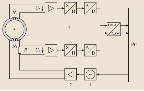
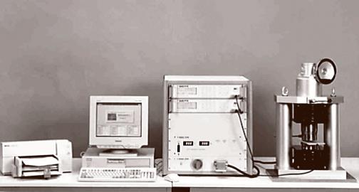
AC Hysteresisgraph
Img src
Programmable function generators allow the waveform of B to be defined as sinusoidal. A sinusoidal H can be easier achieved using a current output amplifier. Systems with digital control for B are available up to frequencies of several kHz, while uncontrolled systems can reach several 100 kHz.
Due to an increase of applications for soft magnetic materials using pulse-width modulation (PWM), the interest in measuring systems that allow measurements in the presence of higher harmonics is growing. Function generators with arbitrarily programmable waveforms can meet these requirements.
Prior to a measurement, the specimen is demagnetized by applying an alternating current with decreasing amplitude.
The AC hysteresisgraph can also measure the curve of normal magnetization. Therefore the amplitude of the magnetizing current is successively increased and corresponding peak values of the field strength and flux density, H and B, are plotted.
An AC hysteresisgraph is mainly used for ring specimens but also sometimes with fixtures that allow measurements of stripes.
Article src: Handbook of Materials Measurement Methods, Horst Czichos, Tetsuya Saito, Leslie Smith, Springer Science+Business Media, 2006.
AC Susceptometry
Img src
AC susceptometry is used in many magnetic nanoparticles applications such as magnetic biodetection, magnetic hyperthermia, magnetic characterization of magnetic nanoparticles and studies of particle stability. In order to gain as much knowledge as possible it is of great importance to both have high magnetic sensitivity and a large excitation frequency range so that it is possible to cover all the magnetic relaxations that are present in a magnetic nanoparticles system, for instance the Brownian and Neel relaxation processes. High frequency AC susceptometers have earlier been reported using toroidal shaped high permeability material or induction techniques. With the toroidal shaped AC susceptometry systems it is possible to reach up to the GHz range but the magnetic sensitivity is low, the sample mounting it is somewhat complicated and it is very important to clean the measurement slit in the toroid minutely in order to have an accurate background response. For induction techniques AC susceptometers the highest reported measurement frequency is in the range of 1 MHz. By using the induction technique with well balanced detection coil system the magnetic sensitivity can be very high, the sample mounting can be easy and the background measurements can be accurate.
AC susceptometer Imego can today measure dynamic magnetic properties from 25 kHz to 10 MHz combined with a high magnetic sensitivity. Thus, together with the medium frequency range DynoMag system we can measure AC susceptibility in the frequency range from a few Hz up to 10 MHz with a very high sensitivity. In the developed AC susceptometers at Imego we use ordinary induction coil techniques with well balanced differential coils in the centre of an excitation coil and sample movement between in the detection coil system.
AC susceptometry based on induction techniques is a valuable magnetic characterization tool for magnetic nanoparticles for instance within the fields of magnetic hyperthermia and for dynamic magnetic analysis of magnetic nanoparticles. When the proper non-linear field dependence of the magnetization is taken into account SHP (Specific Heat Power) values can be estimated from the AC susceptometry analysis with good accuracy when compared to measured SHP values. When the full high frequency AC susceptometer response is analyzed for nanoparticles undergoing Néel’s relaxation, the particle sizes can be estimated or the magnetic anisotropy if the particle sizes are known from other independent analysis techniques for instance size analysis from VSM data.
Article src: DOI : 10.1063/1.3530015
Alternating (Field) Gradient Magnetometer

Img src
The alternating (field) gradient magnetometer (AGM or AFGM) is a modification of the well-known Faraday balance that determines the magnetic moment of a sample by measuring the force exerted on a magnetic dipole by a magnetic field gradient.
The force is measured by mounting the sample on a piezoelectric bimorph, which creates a voltage proportional to the elastic deformation and, hence, to the force acting on the sample. By driving an alternating current through the gradient coils, with lock-in detection of the piezo voltage and by tuning the frequency of the field gradient to the mechanical resonance of the sample mounted on the piezoelectric element by a glass capillary a very high sensitivity can be achieved that approaches that of a SQUID magnetometer under favorable conditions. The main advantage of the AGM is its relative immunity to external magnetic noise and the resulting high signal-to-noise ratio and short measuring time. A major disadvantage is the difficulty in obtaining an absolute calibration of the magnetic moment because the signal is not only proportional to the sample magnetic moment but also to the Q-factor of the sample–capillary–piezo system, which varies with sample mass and temperature.
This problem can be overcome by inserting a small calibration coil close to the sample position. Also, difficulty in obtaining an exact angular orientation of the sample relative to the external magnetic field is a drawback of this instrument. An AGM is relatively easy to build, but is also commercially available. It can be equipped with a cryostat or oven for variable temperature measurements.
Article src: Handbook of Materials Measurement Methods, Horst Czichos, Tetsuya Saito, Leslie Smith, Springer Science+Business Media, 2006.
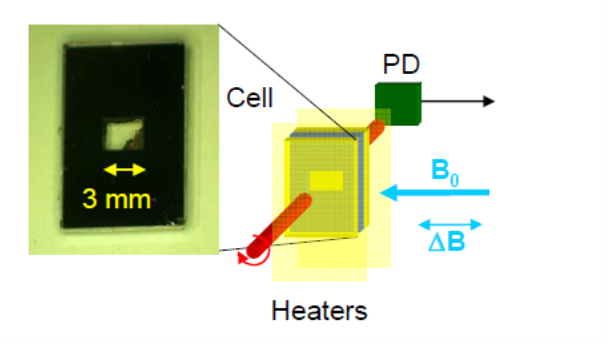
Atomic Magnetometer
Img src
Biomagnetism involves measurement of extremely weak magnetic fields originating from biological systems, including the human body. The most important and most extensively investigated biomagnetism signals are the magnetoencephalogram (MEG) and the magnetocardiogram (MCG), which are the magnetic analogs of the EEG and ECG, respectively. The study of biomagnetism was enabled by the advent of the superconducting quantum interference device (SQUID) magnetometer in the 1960s, and SQUIDs are still the most sensitive commercially available magnetic field detectors. In recent years, however, atomic magnetometer (AM) technology has advanced significantly, and laboratory prototypes with sensitivity exceeding that of SQUID magnetometers have been demonstrated. A major advantage of the AM over SQUID magnetometers is that the AM does not require cryogenic cooling. By eliminating the need for complex, expensive cryogenic equipment, AMs can drastically reduce the cost of MEG/MCG instrumentation. AMs based on alkali atoms enclosed within a vapor cell were first developed in the 1950’s. In 1969, Dupont-Roc and coworkers developed a zero-field version of this AM with nearly 10 fT/√Hz level sensitivity. In 1973, Tang and coworkers discovered a phenomenon, which led to suppression of spin exchange relaxation in alkali atoms, opening a pathway to miniaturization of highly sensitive AMs operating in a low magnetic field. In 2003, Romalis and coworkers used this discovery to demonstrate an ultra-sensitive AM with sub-femtotesla level sensitivity. The AMs operating in this regime are now referred to as Spin-Exchange Relaxation-Free (SERF) magnetometers. In 2007, Shah and coworkers developed a compact version of the SERF AM, using a millimeter-scale microfabricated vapor cell and the simplified detection scheme developed by Dupont-Roc and coworkers. Recently, a fully integrated version of the SERF chip-scale atomic magnetometer (CSAM) was developed at the National Institute of Standards and Technology (NIST). Here we describe a low-cost, compact AM that is a viable alternative to a SQUID magnetometer for biomagnetism applications requiring compact sensors with high sensitivity. Until now, AMs either lacked sufficient sensitivity or were too large and complex for clinical applications. The AMs described here have size and sensitivity similar to that of SQUID magnetometers, and they are manufactured using commercial off-the-shelf components with simple assembly techniques. They also have a precisely defined sensitive axis and can be integrated into a large, dense array for MEG source localization applications; thus, they are suitable as a low-cost, drop-in replacement for SQUID magnetometers in biomagnetism instrumentation.
Article src: A compact, high performance atomic magnetometer for biomedical applications, V. K. Shah & R. T. Wakai, Phys. Med. Biol. 58, 8153–8161, 2013. doi:10.1088/0031-9155/58/22/8153.
Coercimeter

Img src
A coercimeter can be used to determine the coercivity HcJ. As this quantity depends sensitively on the microstructure, it is a good indicator of successful material heat treatment. The measurement is carried out in an open magnetic circuit.
A solenoid is used to magnetize and demagnetize the specimen. The maximum field strength must be sufficient to achieve technical saturation, beyond which the coercivity would remain constant if the magnetizing field strength were further increased. This can be tested by a series of measurements with increasing magnetizing field strengths. The required field strength depends on the specimen material and shape. Commercial solenoids provide up to 100–200 kA/m. Sometimes an additional higher-field pulse is used for saturation.
It is often claimed that coercimeters allow measurement of the coercivity independently of the specimen shape. For machined components such as parts of relays the coercivity is not uniform due to mechanical or heat treatment. Complex-shaped parts are not uniformly magnetized. In these cases the coercimeter provides only an integral value given by the vanishing stray field at the sensor position.
Article src: Handbook of Materials Measurement Methods, Horst Czichos, Tetsuya Saito, Leslie Smith, Springer Science+Business Media, 2006.
DC Hysteresisgraph or Permeameter
Img src
The DC hysteresisgraph or permeameter is used for quasistatic hysteresis measurements on soft magnetic materials. The specimen can either be a bar with round or rectangular cross section or a strip of flat material. The choice of the method depends on the shape and magnetic properties of the specimen. Yoke methods are generally used instead of the ring method if the coercivity of the specimen material is larger than 50–100A/m. Maximum field strengths range from 50–200 kA/m.
The most widespread yoke configurations today are the permeameter yokes type A and type B. Many other, often similar, configurations have been designed. For the measurement of the flux density B, a coil that is directly wound onto the specimen can be used. In everyday use J-compensated coils are often preferred. They can be made more sturdy and can be used for specimens with various diameters and shapes.
In the type A permeameter, the specimen is surrounded by the magnetizing coil. This configuration generates relatively high field strengths.
The type B permeameter uses specimens that are only 90mm long, but the maximum field strength is limited to 50–60 kA/m.
Article src: Handbook of Materials Measurement Methods, Horst Czichos, Tetsuya Saito, Leslie Smith, Springer Science+Business Media, 2006.
Electron paramagnetic resonance (EPR)

Img src
An EPR spectrum is measured by sweeping the external magnetic field applied to the sample placed in a microwave cavity resonant at a fixed frequency of ≈ 10 GHz. Usually the signal is detected by a magnetic field modulation technique so that the resonance field is accurately determined as the fields at which the signal crosses the zero base line. An historical example in which the EPR method shows its power is seen in structural determination of vacancies in Si in different charge states.
One major drawback of EPR spectroscopy is the low resolution (Δν ≈ 10 MHz) compared to NMR (Δν ≈ 50 kHz), which is a disadvantage in the analysis of crowded or overlapped signals. Due to the electron–nuclear interaction, the EPR intensity of each super-hyperfine structure changes when nuclear magnetic resonance occurs in the nucleus responsible for the super-hyperfine EPR signal. This EPR-detected NMR spectroscopy is called electron nuclear double resonance (ENDOR) which also improves the low sensitivity of conventional NMR. ENDOR is used to investigate the spatial extent of the electron cloud probed by EPR.
In semiconductors, unpaired spins as sparse as 1014 to 1016 cm−3 can be detected by EPR provided that the density of free carriers is below 1018 cm−3 so that the microwave can penetrate the sample well. In metals, the presence of free electrons limits the penetration depth below the sample surface due to the skin effect. It should be stressed that EPR signals can be detected only when unpaired electrons are present.
Article src: Handbook of Materials Measurement Methods, Horst Czichos, Tetsuya Saito, Leslie Smith, Springer Science+Business Media, 2006.
Ferromagnetic resonance (FMR)

Img src
Along with high saturation magnetization and high permeability, another important property for high-frequency applications is high ferromagnetic resonance (FMR). FMR is defined as the maximum permissible frequency at which the film can be used in an inductive device.
FMR studies and Brillouin light scattering (BLS) have provided us with detailed information
on spin-wave modes in the regime where the wavelengths are long compared to the lattice constant. FMR probes modes in these metals whose wavelength is comparable to the microwave skin depth, the order of a micron. BLS, a spectroscopy confined to the near surface because of the optical skin depth (∼150–200 Å), allows one to probe modes which propagate parallel to the surface with wavelengths of the order of that of visible light, approximately one-half micron. As we shall see, spin-wave modes of such long wavelengths may be described by a phenomenology similar in spirit to the theory of elasticity when it is applied to the description of phonons.
The FMR spectrum will consist of a rather broad line, with line shape controlled by the spatial
Fourier spectrum of the microwave field, which penetrates into the sample. In such experiments, one scans applied field and measures microwave absorption at fixed frequency; one realizes absorption of energy by spin waves over a rather wide range of fields.
There is a vast literature on magnetic resonance. It formed the basis of the fifth age of magnetism, which flowed from understanding the quantum mechanics of angular momentum, and the development of microwaves for radar in the Second World War. The resonant system is an ensemble of free radicals or ions with unpaired electron spins in electron paramagnetic resonance (EPR) – also known as electron spin resonance (ESR). The entire coupled magnetic moment may resonate in ferromagnetic resonance (FMR).
Since the magnetization of the ferromagnet is largely due to the spin moments of the electrons, γ ≈ −(e/me), resonant frequencies for FMR are similar to those for EPR.
The instantaneous field in the sample is uniform in an FMR experiment provided the wavelength of the microwaves is much greater than the sample size. At 10 GHz, λ = 3 cm, so the condition is satisfied for millimetre-size samples. However, the giant-spin assumption of uniform magnetization throughout the sample is not generally valid. Nonlinear magnetostatic modes may be excited.
Article src: Handbook of Materials Measurement Methods, Horst Czichos, Tetsuya Saito, Leslie Smith, Springer Science+Business Media, 2006.
Article src: Magnetism and Magnetic Materials, J. M. D Coey, Cambridge University Press, 2010.
Article src: Handbook of Magnetism and Advanced Magnetic Materials, H. KronmÜller and S. Parkin, Volume 1: Fundamentals and Theory, John Wiley & Sons, 2007.
Helmholtz-coil configurations

Img src
Helmholtz-coil configurations are very common for the measurement of the magnetic dipole moment of permanent magnets. They provide a large region with uniform sensitivity that can be easily accessed from all sides. Long solenoids can also be used. The installation of the coil must be carried out with care. No magnetic or magnetizable parts are allowed in the vicinity of the coil as they would affect the measurement result. Moreover, an AC hysteresisgraph is mainly used for ring specimens but also sometimes with fixtures that allow measurements of stripes. In these cases the feedback yoke, e.g. a C-core, must be laminated to avoid eddy currents. The permeability should be high compared with the permeability of the specimen. For the winding of the ring specimen the same considerations as for the DC ring method apply. Also, the voltmeter–ammeter method allows the determination of the normal magnetization curve and the amplitude permeability. Generally the magnetization is measured using a pickup coil system, which has to be compensated in order to measure the magnetization M instead of the induction B. For this purpose different arrangements of pick-up coils have been developed. Finally, magneto-optic effects (magnetooptic Faraday effect or Kerr effect, MOKE) are very useful when only the shape of the magnetization loop, or the relative variation of the magnetization with temperature, orientation of the external field or another external parameter is of interest.
Article src: Handbook of Materials Measurement Methods, Horst Czichos, Tetsuya Saito, Leslie Smith, Springer Science+Business Media, 2006
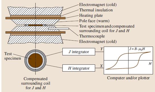
Hysteresisgraph for Hard Magnetic Materials
Img src
A very important instrument for the characterization of bulk permanent magnets is the hysteresisgraph. It is mainly used to record the second-quadrant hysteresis loop. From this, material parameters such as the remanence Br, the maximum energy product (BH)max and the coercive field strengths (coercivities) HcJ and HcB, can be determined. A measurement of recoil loops allows the calculation of the recoil permeability μrec.
Main components use an electromagnet to magnetize and demagnetize the specimen, measuring coils for the field strength H and the polarization J and two electronic integrators (fluxmeters) to integrate the voltages induced in the coils.
An electromagnet with a vertical magnetic-field direction is used. The magnet specimen is placed on the pole cap of the lower pole. The upper pole can be lowered to close the magnetic circuit.
Article src: Handbook of Materials Measurement Methods, Horst Czichos, Tetsuya Saito, Leslie Smith, Springer Science+Business Media, 2006.
Lorentz Force Magnetometers
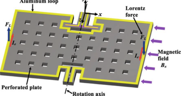
Img src
MEMS-based Lorentz force magnetometers are an alternative for monitoring magnetic field with important advantages such as small size, low power consumption, high sensitivity, good resolution, wide dynamic range, and low cost by using batch fabrication. These magnetometers are small and lightweight compared to SQUIDs devices, search coil sensors, and fiber optic sensors. They could be commercially competitive with respect to anisotropic magnetoresistive (AMR) and giant magnetoresistive (GMR) sensors, and Hall-effect devices. However, MEMS magnetometers need more reliability studies to ensure a safe performance under different environmental conditions.
This structure at resonance can increase the magnetometer sensitivity by a parameter equal to its quality factor. Thus, the magnetic field signal can be converted in electrical or optical signal.
MEMS Lorentz force magnetometers can operate with silicon-based structures, which interact with an external magnetic field and an electrical current to generate a Lorentz force on the structures. This force is perpendicular to the direction of both magnetic field and electrical current. It causes a deformation of the magnetometer structure that can be measured by using a capacitive, piezoresistive, or optical sensing technique. In order to increase the sensitivity of the magnetometer is recommended to operate its structure at resonance. For this, electrical current is applied with a frequency equal to the resonant frequency of the magnetometer structure. This structure at resonance can increase the magnetometer sensitivity by a parameter equal to its quality factor. Thus, the magnetic field signal can be converted in electrical or optical signal.
In addition, different thin films materials can be used in MEMS magnetometers, though, they have properties related with their fabrication
The performance of MEMS magnetometers strongly depends of the functional and structural materials. These magnetometers can have single-crystal silicon (SCS) or polysilicon as materials due to their important electrical and mechanical properties. In addition, different thin films materials can be used in MEMS magnetometers. Although, they have properties related with their fabrication process and post-process such as deposition conditions, annealing, deposition apparatus, and film thickness.
Accurate material properties of MEMS magnetometers should be known to predict their performance. Material properties can be measured using microfabricated test structures on the same wafer. For instance, test structures are used to detect Young’s modulus, Poisson ratio, fracture stress, fracture toughness, fatigue, thermal conductivity, and specific heat measurement.
Article src: Book High Sensitivity Magnetometers, A. Grosz, M. J. Haji-Sheikh, S. C. Mukhopadhyay, Smart Sensors, Measurement and Instrumentation, Springer International Publishing Switzerland, 2017. DOI 10.1007/978-3-319-34070-8
Mx Magnetometer

Img src
The Mx magnetometer configuration is based on a direct optical measurement of the Larmor precession frequency. The atomic spins are pumped into an oriented state with circularly polarized light. A coherent precession about the static magnetic field to be measured is then excited with an applied RF field at the Larmor frequency. The response of the atoms to the drive field is monitored with a probe optical field. In many cases, as is the case here, the pumping and probing can be done with a single optical field that has components lying both along and perpendicular to the magnetic field direction.
Article src: A compact, high performance atomic magnetometer for biomedical applications, V. K. Shah & R. T. Wakai, Phys. Med. Biol. 58, 8153–8161, 2013. doi:10.1088/0031-9155/58/22/8153
Nuclear Magnetic Resonance (NMR)
Img src
NMR spectrometers use superconducting solenoids to provide the bulk magnetic field. While these instruments could be operated in the CW (Continuous Wave) mode, it has proved much more efficient to operate them where the RF (Radio Frequency) is provided through a brief (μs) RF pulse. This excites all of the nuclei simultaneously, and the resulting signals are collected digitally in the time domain (intensity versus time) and then converted to the frequency domain (intensity versus frequency) by Fourier transformation.
While there is a wide range of NMR-active nuclei, only a handful are commonly used. Fortunately, isotopes of the most common atoms in organic molecules are in this category. 1H is the most commonly observed nucleus due to its large natural abundance and high relative sensitivity.
Standard structural analysis by NMR proceeds following
(1) sample preparation, (2) NMR spectra measurements, (3) spectral analysis to assign NMR signals to the responsible nuclei and find the connectivity of the nuclei through bonds and space, (conventionally the term “signals” is used rather than “peaks” because NMR resonances are not always observed as peaks.) and finally (4) the deduction of structural models using the knowledge obtained in (3) as well as information from other chemical analyses as a constraint in the procedure of fitting model to experiment. The final step (4) is like forming a chain of metal rings of various shapes (e.g., amino acid residues in proteins) on a frame having knots in some places linked to others on the chain. For this reason, particularly for macromolecules such as proteins, it is difficult to determine the complete molecular structure uniquely from NMR analysis alone. Since we can only deduce possible candidates for the structure, it is better to refer to “models” rather than “structures.”
This is in marked contrast to structural analysis by Xray diffraction in which the crystal structure is more or less “determined” from the diffraction data alone. Nevertheless, NMR has advantages over X-ray diffraction methods in many respects such as
- Single crystal samples are not needed. The samples may be amorphous or in solution.
- Effects of intermolecular interactions, that may change the molecular structure, can be avoided if samples are dispersed in solution.
- Dynamic motion of molecules can be detected.
- A local structure can be selectively investigated without knowing the whole structure.
- Fatal damage due to intense X-ray irradiation, that is likely to happen in organic molecules, can be avoided.
Article src: Handbook of Materials Measurement Methods, Horst Czichos, Tetsuya Saito, Leslie Smith, Springer Science+Business Media, 2006.
Piezoelectric crystal sensors

Img src
A typical piezoelectric transducer deflects by only 0.001mm under a force of 10 kN. The high frequency response, typically up to 100 kHz due to the high stiffness, makes piezoelectric crystal sensors very suitable for dynamic measurements. The typical range of rated capacities for piezoelectric crystal force transducers is from a few N to 100 MN, with a typical total uncertainty of 0.3% to 1% of full scale. While piezoelectric transducers are ideally suited to dynamic measurements, they cannot perform truly static measurements because there is a small leakage of charge inherent in the charge amplifier, which causes a drift of the output voltage even with a constant applied force.
Piezoelectric sensors are suitable for measurements in laboratories as well as in industrial settings because of their small dimensions, the very wide measuring range, rugged packaging, and their insensitivity to overload (typically by > 100% of full scale). They can operate over a wide temperature range (up to 350 ◦C) and can be packed to form multicomponent transducers (dynamometers) to measure forces in two or three orthogonal directions.
Article src: Handbook of Materials Measurement Methods, Horst Czichos, Tetsuya Saito, Leslie Smith, Springer Science+Business Media, 2006.
Polar Kerr Magnetometer

Img src
Various types of polar Kerr magnetometer have been commercialized, and the fundamental procedures of data gathering, analyses and the sweeping mode of the magnetic field are automatized. It is known that the magneto-optical effect depends strongly on the optical wavelength. For the evaluation of the wavelength dependence, equipment that can cover a wide wavelength range from the ultraviolet to the infrared has been developed and commercialized.
The Curie point is an important factor that is closely relating to the recording sensitivity of MO disks. This value can be obtained by measuring the thermal dependence of the magnetization and the Kerr rotation angle at temperatures varying from the ferromagnetic to the paramagnetic state. The measurements are carries out using the VSM and a Kerr magnetometer with a heating mechanism and thermal monitoring capability.
Article src: Handbook of Materials Measurement Methods, Horst Czichos, Tetsuya Saito, Leslie Smith, Springer Science+Business Media, 2006.
Proton magnetometer
Img src
PM is a magnetic field detection instrument which uses the nuclear (proton) Zeeman effects. It is mainly used for the detection of static or quasi-static weak magnetic fields in the range of geomagnetic field. There are two types of PM: ordinary and dynamic nuclear polarization (DNP). The differences of them lie in different exciting modes and different working substances. The working substance of the ordinary PM is a proton rich solution, such as aviation kerosene, where protons in the solution are directly excited by the direct-current (DC) magnetic field; the sample solution in the DNP magnetometer sensor is a mixture of free-radicals and a proton rich liquids. When working, the free radicals which in the solution is firstly polarized by the radiofrequency (RF) magnetic field, the protons in the solution are then excited by polarized free-radicals. After the polarization condition is removed, the polarized protons will precession with angular frequency x in the target magnetic field, the precession frequency is called Larmor frequency which is proportional to the intensity of the magnetic field, and the target magnetic field will be obtained by measuring the Larmor frequency. The output signal amplitude of Larmor frequency is extremely weak, its maximum value is about microvolt level. Moreover, the signal decays exponentially with time, and it will be drowned by noise within one second, which means that the SNR is very low when the signal is amplified. Therefore, how to obtain accurately the low SNR Larmor frequency is a key issue to improve the precision of PM.
Article src: Microfabricated Atomic Magnetometers and Applications, J. Kitching, S. Knappe, V. Shah, P. Schwindt, C. Griffith, R. Jimenez & J. Preusser, National Institute of Standards and Technology, 2008 IEEE. DOI:10.1109/FREQ.2008.4623107
Article src: A frequency measurement method based on optimal multi-average for increasing proton magnetometer measurement precision, C. Tan, J. Wang & Z. Li, Measurement 135, 418–423, 2019. https://doi.org/10.1016/j.
Pulsed Field Magnetometer (PFM)
Img src
PFM is a instrument that is well suited for fast and reliable measurement of the hysteresis loops of hard magnetic materials.
PFM measurements of hard magnetic materials are reliable and achieve a similar accuracy to that of a static system. In terms of the demagnetizing field, correction for industrial shapes is not simple. For shapes like cylinders or cubes that are not too complex the use of a single factor is sufficient, but for other shapes this problem is still open. This is not only a problem for PFM, but occurs in all magnetic open circuits.
PFMs can be constructed that show better results then many static hysteresisgraphs however with the advantage that in a PFM higher fields are available, a faster measurement is possible and no special sample preparation is generally necessary.
The pulse magnet has to be optimized with respect to the available power, the heating of the magnet and the stresses. The field homogeneity over the desired length of the experiment should be better than 1%. In systems where the hysteresis loop is measured, the pulse magnet has to be optimized with respect to low damping and also for a certain measuring task (maximum field, pulse duration, pulse shape, sample volume).
Generally the magnetization is measured using a pickup coil system, which has to be compensated in order to measure the magnetization M instead of the induction B.
For an industrial system a reasonable sample size is important; typical values are samples up to 30mm in diameter and 10mm in length within a ±1% pick-up homogeneity range. For magnetic measurements exact positioning (reproducibility better than 0.1mm) in the PFM is necessary.
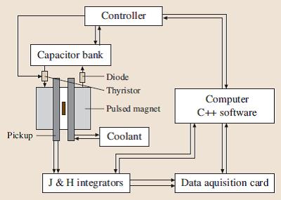
Block diagram of a typical capacitor-driven industrial PFM
A pulsed field magnetometer consists of:
- the energy source, generally a capacitor battery; the stored energy is given by CV2/2. The maximum charging voltage can be 1–30 kV. The capacitance determines the costs of such a system, the maximum sample size and the time constant. For a magnetometer that can measure the full loop, voltage reversal on the battery must be allowed.
- the charging unit, which should generate a reproducible and selectable charging voltage; it determines the repeatability of the achieved field in the pulse magnet.
- pulse magnet: for an existing energy, the pulse magnet determines, via its inductivity, the pulse duration. Additionally the volume (diameter, homogeneity) limits the dimensions of the experiment inside of the magnet. Heating during a pulse may be also a problem when high repetition rates are desired.
- measuring device: this consist of the pick-up system and the measuring electronics (amplifiers, integrators, PCs, data storage). A careful design of the pick-up system is very important in order to achieve a high degree of compensation and consequently a good sensitivity.
- electronics: this consist either of a digital measuring card or of a storage oscilloscope which is connected to a modern data-acquisition system on a standard PC, which allows a software-supported operation of the PFM (charging, discharging and the measurement with an evaluation of the resulting loop).
Article src: Handbook of Materials Measurement Methods, Horst Czichos, Tetsuya Saito, Leslie Smith, Springer Science+Business Media, 2006.
Saturation Coil or Saturation Magnetometer

Img src
The saturation coil, sometimes also called Js-coil or saturation magnetometer, combines the moment-measuring coil with a permanent-magnet system that magnetizes soft magnetic specimens. The measuring coil, usually a Helmholtz coil, is connected to a fluxmeter.
When a specimen with volume V is inserted into the coil, it is magnetized and the magnetic dipole moment j can be obtained from the flux measurement using. If the field strength is sufficiently high, the saturation polarization can be determined through.
Of course the specimen can also be withdrawn from the coil for measurement, but the rotation method, which is frequently used with the moment-measuring coil, cannot
be used. For lower field strength the relative permeability can be calculated using

The inner field strength Hi of the specimen must be determined from the magnetizing field strength, taking into account the demagnetization factor.
The main applications of the method are the determination of the saturation polarization of specimens made of nickel or nickel alloys and the determination of the cobalt content in hard metal specimens.

Article src: Handbook of Materials Measurement Methods, Horst Czichos, Tetsuya Saito, Leslie Smith, Springer Science+Business Media, 2006.
SERF Magnetometer
Img src
This type of magnetometry, known as spin-exchange relaxation free (SERF) magnetometry occurs at very high cell temperatures and very weak magnetic fields.
The sensitivity of most atomic magnetometers is limited ultimately by alkali-alkali collisions. Since the signal from the atoms is proportional to the number of atoms, at low alkali densities the signal-to-noise ratio, and hence the sensitivity, improves as the atom density (at fixed cell volume) increases. However, at a certain density, alkali-alkali spin-exchange or spin-destruction collisions begin to broaden the magnetic resonance, and any gains in sensitivity created by the increased atom number are offset by the correspondingly broader resonance. In 1973, it was discovered that when the density of alkali atoms is very high and the Larmor precession frequency very small (weak magnetic fields), the alkali spins no longer relax due to spin exchange but only via much weaker spin-destruction processes. This effect was used recently to great advantage in magnetometry: the suppression of spin-exchange broadening can lead in the case of 39K to magnetometer sensitivities up to one hundred times better than can be achieved under spin-exchange-broadened conditions. This type of magnetometry, know as spin-exchange relaxation free (SERF) magnetometry occurs at very high cell temperatures and very weak magnetic fields.
The sensitivity of this instrument was less than 70 fT/√Hz at a signal frequency of about 100 Hz. This sensitivity, while still a factor of 50 worse than that of the best atomic and SQUID-based magnetometers, compares favorably with high-Tc SQUID magnetometers. However, the small potential size of this instrument and simplicity of its implementation make it appealing for some applications such as inexpensive, widely deployed magnetocardiological systems. Some improvements in the sensitivity will likely be required before such an instrument could find use in magnetoencephalographic systems.
Another feature of the chip-scale SERF magnetometer (and more generally of all SERF magnetometers constructed so far) is that it appears to operate as a vector magnetometer, being sensitive only to the components of the magnetic field perpendicular to the optical axis. This and the requirement for operation in low fields suggests that these types of magnetometers will be most useful in shielded environments.
Article src: A compact, high performance atomic magnetometer for biomedical applications, V. K. Shah & R. T. Wakai, Phys. Med. Biol. 58, 8153–8161, 2013. doi:10.1088/0031-9155/58/22/8153
Article src: Microfabricated Atomic Magnetometers and Applications, J. Kitching, S. Knappe, V. Shah, P. Schwindt, C. Griffith, R. Jimenez & J. Preusser, National Institute of Standards and Technology, 2008 IEEE. DOI:10.1109/FREQ.2008.462310
Superconducting Quantum Interference Device (SQUID)
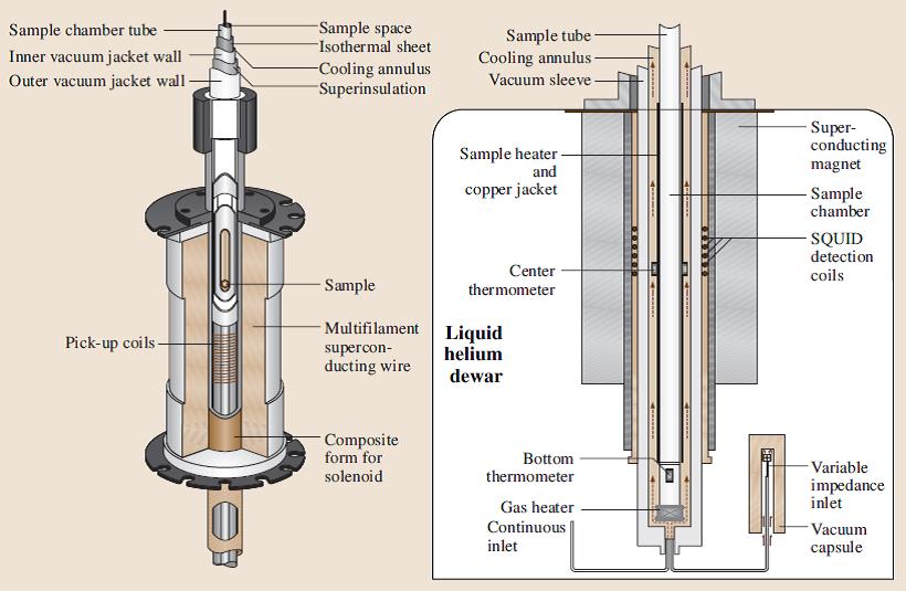
Img src
The SQUID magnetometer is based on the same principle as the VSM but with a superconducting pick-up coil circuit and a superconducting quantum interference device (SQUID) as the flux detector.
10−9 G cm3 or 10−18 V s m.
The detection limit of the SQUID magnetometer for magnetic moments is about 1000 times lower than that of the VSM, i. e. about 10−9 Gcm3 or 10−18 Vsm. It is usually combined with a superconducting magnet and a variable-temperature He cryostat, which allows for measurements in high fields (3–7 T for commercial instruments) and at low temperatures. The biggest challenge is to make use of the high sensitivity of the SQUID in the presence of unavoidable fluctuations of the field from the external magnet. The most efficient solution is to use carefully balanced pick-up coils in the form of a gradiometer of first or second order.
Typical measuring times for a complete magnetization loop may range from 30min up to a full day depending on the field range and number of data points.
For precision measurements a careful calibration that takes into account the specific sample geometry is necessary.
For most purposes the SQUID magnetometer is the most suitable and versatile instrument for measuring extremely thin films in a wide range of temperatures (typically 2–400 K) and applied magnetic fields (up to 7–9T).
Article src: Handbook of Materials Measurement Methods, Horst Czichos, Tetsuya Saito, Leslie Smith, Springer Science+Business Media, 2006.
Torque Magnetometer
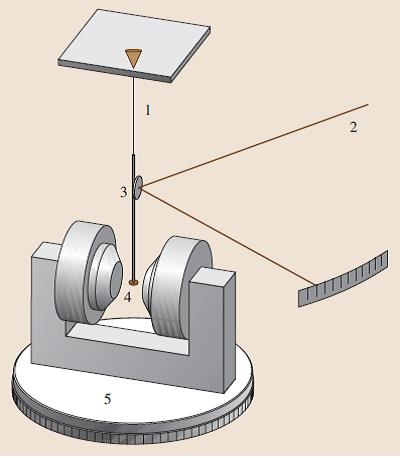
Img src
Torque magnetometers in the form of a torsion pendulum have been successfully used for ultrathin films due to the high sensitivity attainable. However, they measure the effective magnetic anisotropy of the sample; therefore, the different contributions to the anisotropy of the given sample must be known in order to determine the magnetic moment.
The main application of the torque magnetometer is the determination of anisotropy field constants of hard magnetic materials, including small particles and thin films. Other applications are the determination of texture on grain-oriented electrical sheet and tape and the determination of the anisotropy of susceptibility of paramagnetic materials with noncubic structure.
Article src: Handbook of Materials Measurement Methods, Horst Czichos, Tetsuya Saito, Leslie Smith, Springer Science+Business Media, 2006.
Vibrating-Sample Magnetometer (VSM)
Img src
The VSM is used to measure the magnetic moment m and the magnetic dipole moment j = μ0m in the presence of a static or slowly changing external magnetic field. As the measurement is carried out in an open magnetic circuit the demagnetization factor of the specimen must be considered.
Most instruments use stationary pick-up coils and a vibrating specimen but arrangements with vibrating coils and rigidly mounted specimens have also been proposed. The drive is either carried out by an electric motor or by a transducer similar to a loudspeaker system.
The specimen is suspended between the poles of the electromagnet and oscillates vertically to the field direction; it must be carefully centered between the pickup coils.
In the pick-up coils a signal at the vibration frequency is induced. This signal is proportional to the magnetic dipole moment of the specimen but also to vibration amplitude and frequency. The coil design ensures that it is independent of variations in the field generated by the electromagnet.
A VSM is mostly used for measurements on magnetically hard or semi-hard materials. Specimen forms include small bulk samples, powders, melt-spun ribbons and thin films. The VSM can also be used for measurements on soft magnetic materials. In this case the electromagnet can be replaced by a Helmholtz-coil system.
VSMs are very sensitive instruments. Commercial systems offer measuring capabilities down to approximately 10−9 Am2.
A system that used a SQUID sensor instead of pick-up coils achieved a resolution of 10−12 Am2.
Closely related to the VSM is the alternating gradient field magnetometer (AGM). As it is typically used for measurements on thin films.
The VSM allows relatively fast measurements (1–10min for a complete M(H) loop, depending on the type of magnet and the required sensitivity), is flexible and easy to use. In particular, measurements at various angles can be made with the great precision required for the determination of magnetic anisotropies. The sensitivity attainable depends largely on the geometry and position of the pick-up coils. Standard versions are useful for magnetic moments corresponding to Fe or NiFe films more than 5 nm thick (assuming a lateral size of 1–2 cm). Thinner films down to 1 nm can be measured with an optimized VSM. The sensitivity is generally reduced for variable-temperature measurements when a cryostat or oven must be mounted.
For the generation of the outer magnetic field a strong electromagnet is required; the field direction is horizontal. Water-cooled magnets are mostly used but superconducting magnets are also common. The power required is even higher than for a hysteresisgraph as the volume between the pole caps is quite large. The specimen rod must be able to oscillate, and sufficient space for a pick-up coil system is required between the specimen holder and the pole caps.
Article src: Handbook of Materials Measurement Methods, Horst Czichos, Tetsuya Saito, Leslie Smith, Springer Science+Business Media, 2006.