What and how to measure - Metrology

Metrology is generally defined as the “science of measurement.” This, of course, includes its application to a huge range of measurements in science, industry, the environment, as well as in healthcare or food quality; metrology is all around each and every one of us. Measurement provides us with a reference for our daily life in the measurement of time, weight, length and all the hundreds of measurements that influence us.

The emergence of quantum-based standards, was an important and highly significant development. In retrospect, these were one of the drivers for change in the way in which world metrology organizes itself and had implications nationally as well as internationally.

For coordinating world metrology, the website of the Bureau International des Poids et Mesures (BIPM) recognized the need to develop a world metrology infrastructure in new areas such as the environment, chemistry, medicine and food.

Industry presses National Metrology Institute (NMIs) for better performance and in some areas of real practical need. NMI measurement capabilities are still rather close to what industry requires.

Article src: Handbook of Materials Measurement Methods, Horst Czichos, Tetsuya Saito, Leslie Smith, Springer Science+Business Media, 2006.

During the past 100 years many different methods have been developed for the measurement of magnetic material properties and sophisticated fixtures, yokes and coil systems have been designed. Many of them vanished when new materials required extended measuring conditions. With progress in electronic measuring techniques some instruments were replaced. Fluxmeters and Hall-effect field-strength meters, for example, replaced ballistic galvanometers and rotating coils. New methods are ready to enter magnetic measuring technique. One new opportunity is for the pulse field magnetometer (PFM). This device can complement the capabilities of a hysteresisgraph for hard magnetic materials, although it should be mentioned that the instrumentation is not less demanding. The difficulties involved require a careful interpretation of the results.

Some basic methods in magnetic measurement are taken as known. Fluxmeters are used in many measuring set ups to integrate voltages that are induced in measuring coils to obtain the magnetic flux. Today various analog or digital integration methods are used. The same applies for field-strength meters that use the Hall effect. These instruments, usually called Gauss or Teslameters, are widespread. In many cases it is impossible to determine the material properties of components in a shape that is defined by the production conditions or application. In these cases, relative measuring methods are often applied. These usually compare measurable properties or combinations of properties with those of a reference sample.

Basically, almost all of the materials properties such as magnetic properties, are temperature-dependent, except these cases where a material is especially designed to be resistant to temperature variations. For example, temperature influences mechanical hardness, electrical resistance, magnetism, or optical emissivity. Temperature is also of importance to the characterization of material performance as it influences materials integrity when subject to corrosion, friction and wear, biogenic impact or material–environment interactions. However, it should be noted that temperature-dependent measurements are possible, although technically more complex such as in the case of magnetic measurements.

Article src: Handbook of Materials Measurement Methods, Horst Czichos, Tetsuya Saito, Leslie Smith, Springer Science+Business Media, 2006.

Intrinsic magnetic properties are those characteristic of a given material (e.g. spontaneous magnetization, magneto-crystalline anisotropy constant etc.), while extrinsic properties are strongly affected by the specific shape and size of the magnetic object as well as by their microstructure. The most important example is the magnetic shape anisotropy caused by the dipolar energy via the demagnetizing field: for a three-dimensional ferromagnetic object characteristic quantities such as the remanent magnetization and saturation field are mainly determined by the shape and much less by the intrinsic magnetic anisotropy. Another extrinsic effect is the role of mechanical strain in a specimen; this may be introduced during the production process. Stress and strain may significantly alter the shape of the magnetization loop via magnetostrictive effects.

Saturation Magnetization, Spontaneous Magnetization

The saturation magnetization of a material M_sat, defined as the magnetic moment per volume, is of great technical interest because it determines the maximum magnetic flux that can be produced for a given cross section. However, M_sat as the magnetization at technical saturation is not a well-defined quantity because a large enough external magnetic field must be applied to produce a uniform magnetization by eliminating magnetic domains and aligning the magnetization along the

field against magnetic anisotropies; however, at the same time the magnetization at any finite temperature T> 0 will continue to increase with increasing applied field (high-field susceptibility). The only well-defined quantity, hence, is the spontaneous magnetization M_S i. e. the uniform magnetization inside a magnetic domain in zero external field.

In practice, M_S is determined by measuring the magnetization as a function of the external field, M(H) (which means the magnetization component parallel to the applied field) up to technical saturation, with a linear extrapolation of the data within the saturated region back to H = 0. A linear fit is a good approximation for temperatures well below the Curie temperature of the ferromagnetic material.

The method proposed above works best by applying the external field along an easy axis of magnetization and is especially well suited for thin films because of the absence of a demagnetizing field for in-plane magnetization; usually a relatively small field is sufficient for saturation and the extrapolation to H = 0 is not required. Of course, higher fields are required for magnetically hard materials. In films having a dominating intrinsic anisotropy with a perpendicular easy axis the measurement should be done along the film normal.

When comparing the magnetization of a thin film to the value of the corresponding bulk material two different effects can be important:

1. the magnetization or the magnetic moment per atom in the ground state, i. e. at absolute zero temperature, might be enhanced. Depending on the specific combination of ferromagnetic material and substrate the enhancement may reach 30% for a single atomic layer (e.g. Fe on Ag or Au), but will disappear 3–4 atomic layers away from the interface. Depending on the band structure of the materials the magnetic moments at the interface may also be reduced in some cases (e.g. for Ni on Cu);
2. thermal excitations which result in a decrease of M_S with increasing temperature are more pronounced in thin films compared to bulk material. In a film of 10 atomic layers of Fe on Au, M_S at room temperature is reduced by about 10% compared to bulk Fe. The origin of this effect is the reduced (magnetic) coordination at surfaces and interfaces, which leads to an enhanced excitation of spin waves; for the same reason the Curie temperature is reduced in ultrathin films compared to the bulk material.

Time-Dependent Changes in Magnetic Properties

Ferromagnetic materials frequently show a continuous change of their macroscopic magnetization in the course of time even in a constant or zero applied magnetic field. This is usually termed the magnetic aftereffect or magnetic viscosity and may occur on a time scale of seconds, minutes or even thousands of years. The underlying physical reason is that a ferromagnetic object

with a net magnetic moment in the absence of an external magnetic field is generally in a thermodynamically metastable state. This is indicated by the presence of hysteresis. The equilibrium state will be asymptotically approached by domain nucleation and wall motion. Domain-wall motion is a relatively slow process due to the effective mass or inertia that can be attributed to a magnetic wall; since it is thermally activated it, also depends strongly on temperature. For the same reason the coercivity of a sample depends on the measurement time if magnetization reversal occurs via domain walls. This needs to be taken into account when comparing data obtained by quasistatic measurements with those extracted from high-speed measurements.

In the absence of domains walls and for a uniformly magnetized sample the magnetization responds to the torque exerted by an external magnetic field by a precession of the magnetization vector around the effective field, which is well described by the Landau–Lifschitz–Gilbert equation. As a consequence, in these cases the maximum rate of change of the magnetization is limited by the precession frequency of the magnetization vector, which for common materials like Fe, Co, Ni and their alloys is between 1 GHz and 20 GHz in moderate applied magnetic fields. It is evident that magnetization dynamics on a timescale of nanoseconds and below is relevant for magnetic devices in high-frequency applications.

Article src: Handbook of Materials Measurement Methods, Horst Czichos, Tetsuya Saito, Leslie Smith, Springer Science+Business Media, 2006.

The most important magnetic quantities are defined in the following in conjunction with their primary measurement methods.

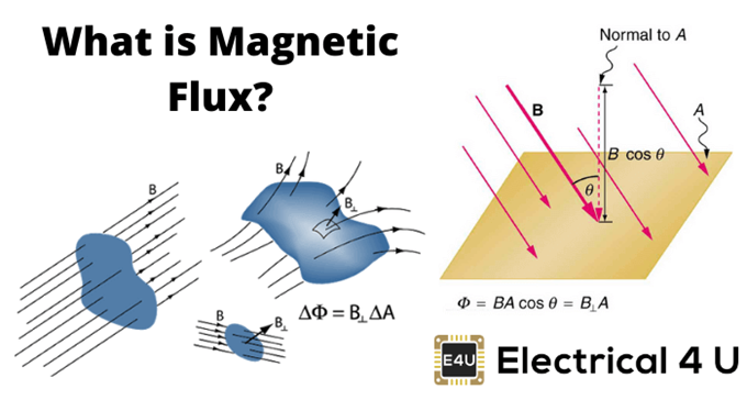
The magnetic field H, or flux density B, (which are equivalent in free space) are measured with Hall probes, inductive probes (e.g. flux-gate magnetometers for very low fields) or nuclear magnetic resonance (NMR) probes for very high accuracy.

Magnetic moments are measured by different types of magnetometers

• via the force exerted by a magnetic field gradient [e.g. Faraday balance, or alternating gradient magnetometer (AGM)]
• via the voltage induced in a pick-up coil by the motion of the sample, e.g. the vibrating-sample magnetometer (VSM) is a widely used standard instrument, or a superconducting quantum interference device (SQUID) magnetometer for highest sensitivity

The (average) magnetization of a magnetic object is usually determined by dividing the magnetic moment by the volume of the sample. Care must also be taken concerning the vector component of the magnetic moment that is detected. This is crucial in the case of samples with a significant magnetic anisotropy which can even result from the shape of the specimen.

All these instruments need careful calibration. This is important because the effective calibration factors depend more or less on the size and shape of the specimen.

Magnetic moments related to different chemical elements in a specimen can be measured selectively by means of magnetic X-ray circular dichroism (MXCD) using circularly polarized X-rays from a suitable synchrotron radiation source. In principle, this method allows the separation of orbital and spin magnetic moments.

If only the a relative value of the magnetization is of interest and not its absolute value, then a number of

different methods can be used to measure, for instance, M as a function of temperature or of the applied magnetic field. Such methods include magneto-optic effects [e.g. the magneto-optic Kerr effect (MOKE)] or the magnetic hyperfine field measured by using the Mößbauer effect, perturbed angular correlations (PAC) of gamma emission, or nuclear magnetic resonance (NMR). While MOKE is widely used for characterizing magnetic materials, nuclear methods due to their relative complexity are restricted to special applications where standard techniques do not provide adequate information.

Article src: Handbook of Materials Measurement Methods, Horst Czichos, Tetsuya Saito, Leslie Smith, Springer Science+Business Media, 2006.

The magnetic calibration corrects for any constant offset to the applied and the measured magnetic fields.

Field Calibration

The field is calibrated using a small pick-up coil whose effective winding area is known from an NMR calibration. The induced voltage u(t) is then fitted using,

in order to determine the field calibration factor k, the damping factor α and the pulse duration (including the effect of the damping). Using such a procedure, an absolute field calibration of better than 1% is achieved.

Magnetization Calibration

The magnetization is calibrated using well-known materials such as Fe and Ni (in which the eddy-current error causes an uncertainty) or preferably a nonconducting sample such as Fe₃O₄. All calibration measurements are performed at room temperature as summarized in the following table. To check the reproducibility all measurements were repeated 10 times to give an average value<M>. For the metallic samples an error of 1–2% due to the eddy currents occurs. The mean value of the deviations D_mv = 1.6% is higher than the true values. The mean value of the deviations D_mv = 1.6%  has a standard deviation of 0.95%. The standard deviations concerning the reproducibility gave a mean value of 0.19%. Therefore, the deviation is, in the worst case, 1.14%. This means that the magnetization value could be calibrated with an absolute accurately of ±1.14%.

Table 10.3 Summary of calibration results

10.10 L. R. Moskowitz: Permamnent Magnet Design and Application Handbook (Cahners Books International, Boston 1976) pp. 128–131

10.11 G. Bertotti, E. Ferrara, F. Fiorillo, M. Pasquale: Loss measurements on amorphous alloys under sinusoidal and distorted induction waveform using

a digital feedback technique, J. Appl. Phys. 73, 5375–5377 (1993)

10.12 D. Son, J. D. Sievert, Y. Cho: Core loss measurements including higher harmonics of magnetic induction in electrical steel, J. Magn. Magn. Mater. 160, 65–67 (1996)

Reliability

For testing the reliability of the calibration procedure, a “reference sample” with “known” features may be used and if the difference between the measured and the literature values is less than the given calibration error (i.e. <1%), such evidence strongly supports the reliability of  calibration process.

Article src: Handbook of Materials Measurement Methods, Horst Czichos, Tetsuya Saito, Leslie Smith, Springer Science+Business Media, 2006.

In order to obtain the coercive field of the specimen under fields with different sweep rates, hysteresis loops of the samples are recorded at a fixed temperature by using a pulse field magnetometer (PFM) applying a sufficiently high maximum field. The sweep rate dH/dt can be changed either by varying the capacitance of the condenser battery or by changing the amplitude of the field or both;

Powder samples can be measured in the same way as solid magnets if the powder is filled into a nonmagnetic container, for example a brass ring that is sealed with a thin adhesive foil at the bottom.

Generally, the magnetocrystalline anisotropy constants may be determined from measurements on a single crystal in a torque magnetometer or similar device. Unfortunately, single crystals are not available from many materials. In this case, polycrystalline material can sometimes be aligned in an external field and then the magnetization M(H) is measured parallel and perpendicular to the external field. Curves determined in this way can be fitted, which also allows an estimate of the magnetocrystalline anisotropy to be made.

Sample Geometry

The effect of the sample geometry on the accuracy a set of industrial soft magnetic ferrites (3C30 Philips) with different shapes is outlined. This material has a magnetization at room temperature of about 0.55 T, whilst the Curie temperature is about 240 ^oC. The density is 4800 kg/m³. Since this material is an insulator, there are no eddy-current effects. All samples are measured in a PFM at room temperature (21 ◦C±1 ◦C) using similar conditions with an amplitude of 2 T and a pulse duration of 56 ms. The magnetization values of the three different cubes show a difference of up to 0.6%. The value for the sphere exhibits the largest difference of 2% with respect to the average value of the cubes.

Magnetization, shapes and masses of the 3C30 samples at H = 2 T of 3C30 samples

Constraints

Eddy-currents: The application of a transient field causes eddy currents in metallic samples which lead to a dynamic magnetization M_eddy that is proportional to dH/dt; the proportionality factor is the specific electrical conductivity. Additionally, M_eddy scales with R² (R is the radius of a rotational symmetrical sample), which means that the error increases quadratically with increasing sample diameter. Fortunately, most of the metallic permanent magnets are sintered materials where the specific resistivity (typically 2×10⁻⁴ Ω m) is generally a factor 50–100 higher that of Cu. Therefore, the error in magnetization measurements due to eddy currents is rather small.

Magnetic viscosity: When the hysteresis loop of hard magnetic materials is measured in transient fields the so-called magnetic viscosity causes a difference between the measured loop and the true loop. The magnetic viscosity is also observed in nonconducting materials (e.g., ferrites), therefore it is not due to eddy currents.

Article src: Handbook of Materials Measurement Methods, Horst Czichos, Tetsuya Saito, Leslie Smith, Springer Science+Business Media, 2006.

Magnetometers can be classified according to different criteria.

Physical effects: Accordingly, magnetometers can be classified as follows: sensors made according to Faraday’s electromagnetic induction law are called induction magnetometers; magnetometers working by the principle that current in the magnetic field can generate a Lorentz force are called magnetic magnetometers; where the resistivity of the conductor changes in the magnetic field, this type of sensor is called a magnetoresistive magnetometer; magnetometers based on the Faraday magneto-optical effect are called magneto-optical magnetometers, such as the optical pump magnetometer; magnetic sensors based on the Josephson effect are called superconducting quantum interference devices (SQUID), etc.

Detection technology: This classification is based on the different measuring methods. Some magnetometers’ physical effects are the same, but they are different in their detection method, which is because the magnetic field measuring methods are built on the basis of various physical effects and physical phenomena related to the magnetic field. There are dozens of methods to measure the magnetic field at present. Some of these are basic, widely used, and have broad development and can be divided into the following types: force and moment method, measuring by the Lorentz force of magnet or carrying fluid acting in the magnetic field; electromagnetic induction method, based on Faraday’s law of induction, can measure DC, AC, and pulse magnetic fields, usually including a ballistic galvanometer, flux meter, electronic integrator, rotation coil magnetometer, vibrating coil magnetometer, etc.; Hall effect method; magnetoresistance effect method; magnetic resonance method, weakly connected superconducting effect method (SQUID); magnetic flux gate method; magneto-optical method; magnetostrictive method; etc.

Spatial measurement: This corresponds to the ability to measure the vector information of the magnetic field, there are vector sensors which are available to measure the magnetic field along the magnetometer sensitivity axis, and scalar (total) sensors, which can only measure the magnitude of the magnetic-field vector. There are also point field sensors that can measure a point of magnetic field information in space and magnetometers that can only measure the average magnetic field information in a certain region in space, which is related to the size of the sensitive element of the magnetometer. However, there are no uniform criteria for this classification. If it is small enough for the size of the sensitive direction of the sensitive element compared to the range measurement, we can consider that it is capable to measurement as a point magnetic field.

Sensitivity: This important classification method, is based on the sensitive range and the sensitive resolution of various specific magnetometers. The magnetic field to be measured can generally be divided into three categories as follows: weak magnetic field (<1 mG=0.1 nT); medium magnetic field (1 mG–10 G); strong magnetic field (>10 G). This classification is based on the intensity of the geomagnetic field. Considering the needs of the task, magnetometers that measure the above magnetic fields are also divided into three types: high-sensitivity magnetometers; medium-sensitivity magnetometers; and low-sensitivity magnetometers.

Article src: https://www.sciencedirect.com/topics/engineering/magnetometer